Statistical Summary "Lumping Up" Rules for Simulation Models


One of the strengths of ARM is the high temporal frequency with which measurements are taken (once every minute for most instruments). Ironically, this strength can also be troublesome, since few simulation models are designed to make use of such fine-scale temporal data sets. Thus, before ARM measurements can be used in carbon models, they must be pre-processed statistically to produce summaries which are of a temporal resolution that is better-matched to the input needs of contemporary carbon simulations.
Another troublesome consideration for modelers is that surface meteorology observations are not made at ARM extended facilities located within about 10 km of existing surface meteorological stations such as those of the Oklahoma MESONET. The Oklahoma MESONET has over 50 surface stations within the boundaries of the SGP site.
Modelers wishing to employ ARM data as meteorological drivers would have to determine the closest Oklahoma MESONET station, obtain this "external" data set, and merge this data stream with the cotemporaneous ARM measurement observations. The data products which we have designed specifically for carbon models have these "external" observations already merged and appropriately summarized, ready for immediate use in carbon simulations.
There is a secondary consideration to this temporal downscaling which may be less obvious. Many contemporary carbon models are designed for daily input values. To supply a daily simulation model which needs a daily minimum temperature with the minimum temperature measurement from an instrument which is measuring every minute may be misleading. A one-minute minimum, although it may be a valid measurement, may not be representative of the daily minimum needed by the simulated processes, since it will capture short transient events which may have little effect on carbon processes. Instead, we define daily minimum temperature as the mean value for the coldest hour. This "lumped-up" definition of daily minimum temperature is more meaningful than a more instantaneous minimum that would be represented by the minimum of the one-minute measurements from each day. Similar logic was extended to representations of maximum values.
The table below provides details of the summarization logic and parameters generated for the carbon model input product (The units of the summaries are identical to the units of the ARM data source).
Description of summarization logic and output parameters.
| Measurement: Summary | hourly | daily | monthly |
| Air temperature: mean | mean of 1 minute values within an hour | mean of 1 minute values within a day | mean of 1 minute values within a month |
| Air temperature: minimum | minimum of 1 minute values within an hour | minimum of hourly means within a day | mean of the daily minimums |
| Air Temperature: hour of the minimum | *** | hour of day for the minimum | *** |
| Air temperature: maximum | maximum of 1 minute values within an hour | maximum of hourly means within a day | mean of the daily maximums |
| Air temperature: hour of the maximum | *** | hour of day for the maximum | *** |
| Air temperature: % of available measurements | The percentage of possible measurements that are available for the calculations. | The percentage of possible measurements that are available for the calculations. | The percentage of possible measurements that are available for the calculations. |
| Precipitation: total | sum of precipitation within an hour | sum of precipitation within a day | sum of precipitation within a month |
| Precipitation: maximum | maximum precipitation within an hour | maximum hourly precipitation total within a day | maximum daily precipitation total within a month |
| Precipitation: % of available measurements | The percentage of possible measurements that are available for the calculations. | The percentage of possible measurements that are available for the calculations. | The percentage of possible measurements that are available for the calculations. |
| Vapor Pressure: mean | mean of 1 minute values within an hour | mean of 1 minute values within a day | mean of 1 minute values within a month |
| Vapor Pressure: minimum | minimum of 1 minute values within an hour | minimum of hourly averages within a day | mean of the daily minimums |
| Vapor Pressure: hour of minimum | *** | hour of day for the minimum | *** |
| Vapor Pressure: maximum | maximum of 1 minute values within an hour | maximum of hourly averages within a day | mean of the daily maximums |
| Vapor Pressure: hour of maxium | *** | hour of day for the maximum | *** |
| Vapor Pressure: % of available measurements | The percentage of possible measurements that are available for the calculations | The percentage of possible measurements that are available for the calculations | The percentage of possible measurements that are available for the calculations |
| Wind Speed : mean | average of 1 minute values within an hour | average of 1 minute values within a day | average of 1 minute values within a month |
| Wind Speed: maximum | maximum of 1 minute values within an hour | maximum of hourly average values within a day | mean of the daily maximums |
| Wind Speed: % of available measurements | The percentage of possible measurements that are available for the calculations | The percentage of possible measurements that are available for the calculations | The percentage of possible measurements that are available for the calulations |
| Wind Speed : mean | average of 1 minute values within an hour | average of 1 minute values within a day | average of 1 minute values within a month |
| Wind Speed: maximum | maximum of 1 minute values within an hour | maximum of hourly average values within a day | mean of the daily maximums |
| Wind Speed: % of available measurements | The percentage of possible measurements that are available for the calculations | The percentage of possible measurements that are available for the calculations | The percentage of possible measurements that are available for the calculations |
| Solar radiation: mean | average of 1 minute values within an hour; only for hours containing values greater than 0 | average of 1 minute values within a day; only including minutes containing values greater than 0 | average of 1 minute values within a month, only including minutes containing values greater than 0 |
| Solar radiation: total | sum of 1 minute values within an hour; include only values greater than 0 | sum of 1 minute values within a day include only values greater than 0 | sum of 1 minute values within a month, include only values greater than 0 |
*** summary not calculated
We have generated a set of hourly- and daily-aggregated data products,
generated as described above, which are specifically designed for easy
implementation of ARM data as drivers in carbon simulations. Because of
the wide variety of carbon simulations that are available and the speed
with which new simulations are constantly being developed, we did not
tailor these data products for use with
Consistent with this general use philosophy, we have been inclusive with regard to the selection of summarized ARM parameters. While it will be rare that any single model will need all of these measurement types, we did not wish to exclude more exotic parameters without which particular models cannot run.
list of files for data products
Browse-o-rama link
README at top of directory listing
ARMish format names explanation
Daily NetCDF files obtained from the ARM archive containing the
finest-grain ARM measurements are the starting point for the statistical
aggregation process. All of these daily NetCDF files for a given year
are combined into an annual NetCDF file using the ncrcat
program which is part of the NCO utility package by Zender. Concatenation is
necessary to allow data summarizations that span more than a single
day (e.g., monthly averages).
The annual NetCDF file is loaded into SAS for summarization.
The ncdump utility is used to generate an ASCII file
from the annual NetCDF file. Then the ASCII file is read into SAS.
The program creates a SAS data set containing an observation for each
measurement taken that year. The program also writes the starting time
and the time step, and adds a date-time field in Greenwich Mean Time to
each observation in the output data set.
The data sets undergo a quality control check. Records are checked for duplicate entries (rare), gaps, and measurement values which are out of bounds. Each measurement is filtered based on quality control limits specified in the NetCDF file header for valid instrument response. These limits are set in coordination with each instrument mentor.
We calculate the local times of sunset and sunrise for each date at each location, and use these as a temporal mask to calculate daytime averages. For example, shortwave measurements are not reliable at night, since the pyranometers emit blackbody radiation after dark. Infrared cooling of the pyranometers at night produces artificial negative fluxes seen in the measurement data, which must be removed before the measurements are suitable for use in carbon models. Some carbon models need average daytime temperature, for which the daylight masks are also used.
Summary statistics are calculated using a specified aggregation interval. We have produced statistics for ARM SMOS and SIRS data sets from 1996 through 2001 aggregated to daily and hourly intervals for all ARM CART locations. As explained above, it may not be prudent to use true maxima and minima as, for example, daily maximum or daily minimum values in a simulation model. Thus, even if your model calls for daily values, you may need the hourly aggregation files.
Summary statistics include the number, minimum, maximum, mean, standard deviation, mode, median, skewness, and kurtosis of the values in the aggregation interval. The values are written to a SAS data set, which is then used to produce a tab-delimited ASCII data set which can easily be used to construct input data sets appropriate for a variety of carbon simulations.
Daily and hourly aggregated data sets are available. There is one ASCII file per site per year. All measured parameters are included in each file, as well as some calculated secondary parameters. There is one record per aggregated time interval. The files are organized so that all records for each parameter are together, followed by all aggregated records for the next parameter, and so on. This organization makes it easier to harvest the values needed for a particular model.
We have filled any data gaps in these daily and hourly aggregated data products using our Univariate Generic Imputation Tool (UGIT), so that the data sets are complete for all parameters and all sites (ARM facilities and Ok MESONET sites). Imputed values can be readily identified, since they carry a flag indicating which type of regression model was used to estimate them, and also because they do not have associated values of calculated statistical properties.
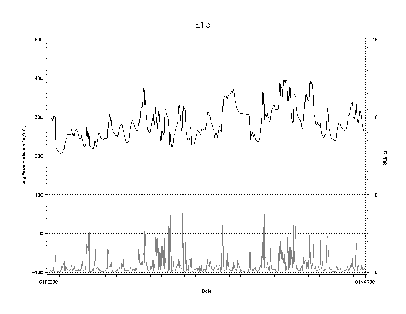
In order to assist and encourage carbon modelers as they "shop" for data appropriate to use in carbon simulations, we have prepared a set of "quicklook" graphs, one for each parameter included in the new data products. Quicklooks plot one year of a single parameter, either daily or hourly. Each quicklook file consists of a single annual plot, followed by 12 monthly plots in greater detail. Standard errors for the parameter are also plotted at the bottom of each graph.
Future synthetic data products from this project will include spatial area estimates of the same sets of parameters distributed here, interpolated between ARM locations. Gap-filling is a special case of such spatial interpolation. Gridded data sets will be appropriate for driving carbon models which are operating in a gridded mode over the entire ARM CART spatial area.

