Predicting Susceptibility of Great Lakes to Aquatic Invasive Species

Introduction

Aquatic invasive species are transported with normal ship traffic, often as ballast water. This study attempts to predict susceptibility by quantifying the degree of multivariate similarity of aquatic environments worldwide to selected locations within the Great Lakes, USA.

Our approach assumes that, sooner or later, transport of invasive aquatic organisms will occur to and from all points on the globe. Following such human-mediated transplantations, it is the degree of similarity of the new aquatic environment to the original environment that determines whether the invader will successfully establish a population in the new location.

Toward this end, we have produced multiple sets of aquatic ecoregions, based on six characteristics of the surface aquatic environment. Using Multivariate Geographic Clustering (MGC) on a parallel supercomputer, we grouped over 50M 4 km map cells into groups or clusters having similar combinations of the six environmental conditions. When placed back into geographic space, these groups form geographic regions which share similar environmental conditions.

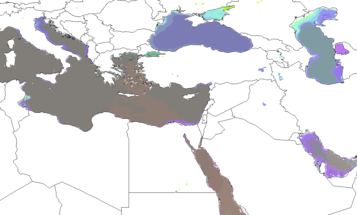
Because the ecoregionalization process is quantitative, we can also compute the degree of similarity between any single aquatic ecoregion or group of aquatic ecoregions and every other aquatic ecoregion in the world. A world map can be drawn in which the degree of multivariate similarity between the aquatic environment in the selected location and the aquatic environment in every other location is shown as a shade of gray.

By quantifying the similarity between aquatic environments, such maps show both the locations from which aquatic invasive organisms that are likely to survive here might come, and locations to which invasive aquatic forms from this location might go and establish a viable population. Using a similarity-based approach, it is not necessary to select a particular donor and recipient location, or to do the analysis on a species-by-species basis.

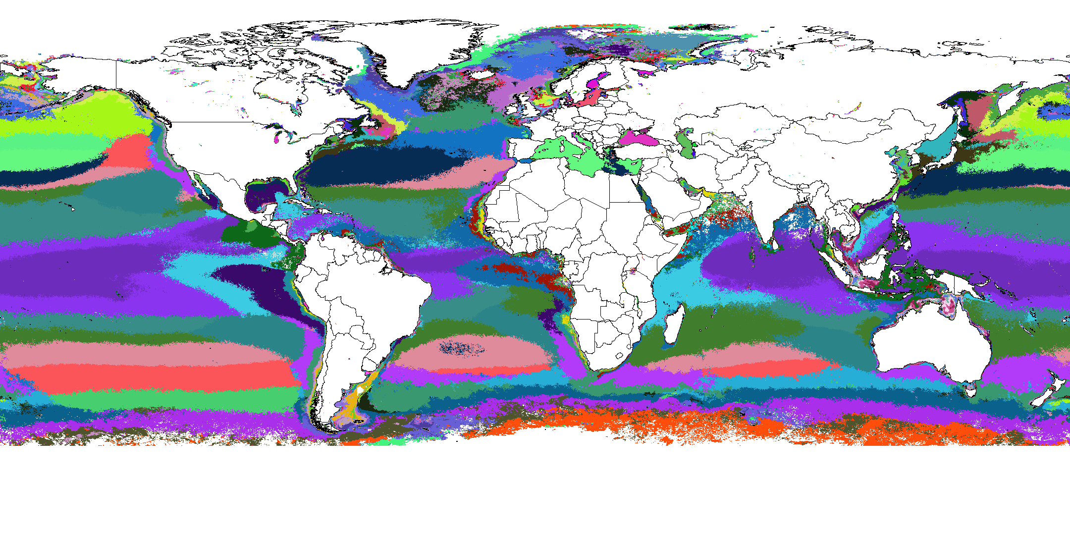
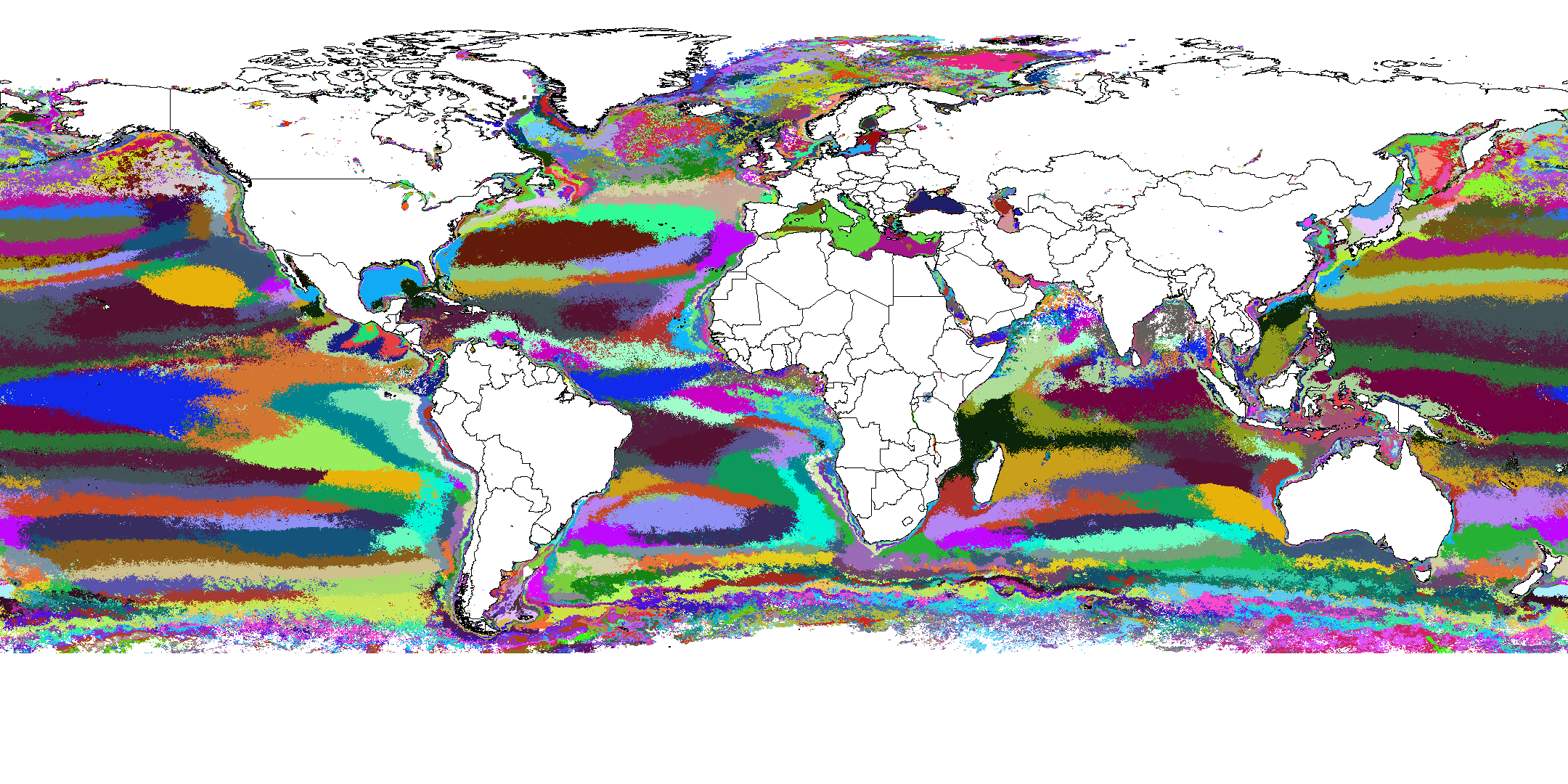
The world map below shows the 1000 most-different global aquatic ecoregions, shown in random colors, based on minimum, maximum, and mean surface water temperature, mk90, nlw551, and chlorophyll content.

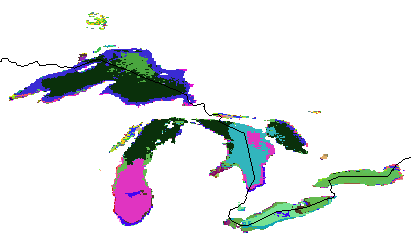
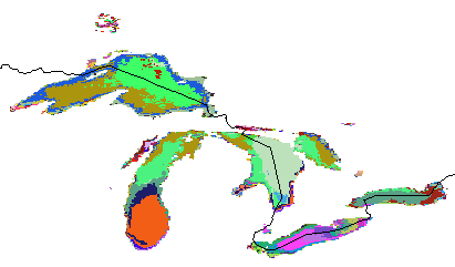
A zoomed map shows the randomly colored aquatic ecoregions found within the Great Lakes.

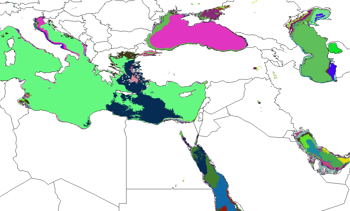
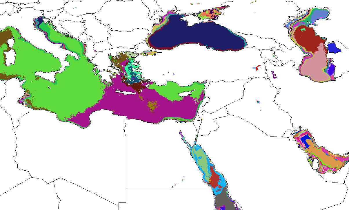
The map of Great Lakes ecoregions can be compared with a zoomed map showing the aquatic ecoregions of the Ponto-Caspian seas, shown in the same random colors. Because they have been put on a common basis for direct comparison, it is easy to see that these two locations share a number of common aquatic ecoregions, and therefore might be susceptible to invasive cross-transport.

Using Similarity Colors to Show Similar Aquatic Environments

Mapping the global aquatic ecoregions in random colors emphasizes the borders between different aquatic ecoregions, but does not show the degree of similarity of environmental conditions between different aquatic ecoregions. It is also possible to statistically generate colors that are proportional to the mix of the six environmental conditions occurring within each aquatic ecoregion. By performing a Principal Component Analysis on the data and generating the first three Principal Component (PC) axes, and then assigning each of those axes to the red, green, and blue color guns, respectively, we can statistically generate a color that reflects the proportional mixture of environmental conditions within each aquatic ecoregion. Using these Similarity Colors, two different aquatic ecoregions having nearly the same mixture of environmental conditions will be shown in nearly the same Similarity color. Simple visual inspection will indicate areas having similar environments.

In this example, PC 1 represents warmth, and is shown in red. PC 2 is chlorophyll and mk90, and is shown in green. PC 3 is nlw551, and is shown in blue.

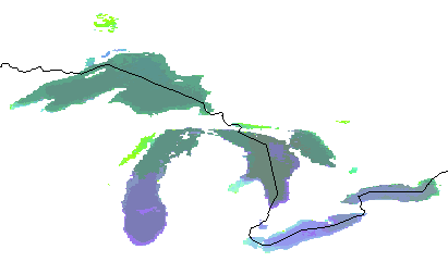
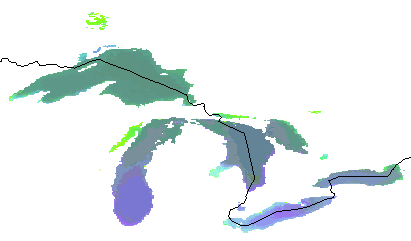
The similarity colored aquatic ecoregions found within the Great Lakes are shown below.

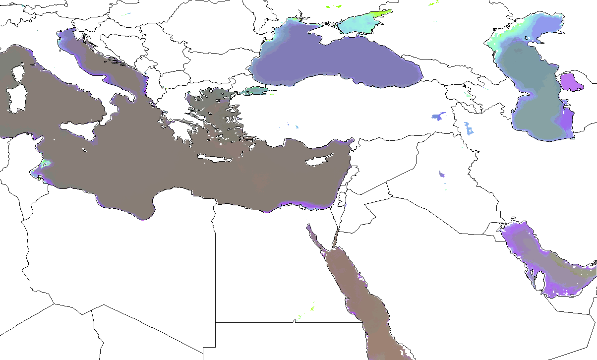
A zoomed map showing the aquatic ecoregions of the Ponto-Caspian seas, shown in similarity colors.

Creating 3000 High-Resolution Global Aquatic Ecoregions

We repeated the global aquatic environments analysis using the same six variables, but statistically delineating the 3000 most-different aquatic ecoregions. The same sequence of maps is shown below based on 3000 worldwide aquatic ecoregions.

The world map below shows the 3000 most-different global aquatic ecoregions, shown in random colors, based on minimum, maximum, and mean surface water temperature, mk90, nlw551, and chlorophyll content.

A zoomed map shows the randomly colored aquatic ecoregions from the 3000-ecoregion set found within the Great Lakes.

The map of Great Lakes ecoregions can be compared with a zoomed map showing the aquatic ecoregions of the Ponto-Caspian seas from the 3000-ecoregion set, shown in the same random colors. When resolved into this many different aquatic ecoregions, few ecoregions are an exact match between the GLs and the Ponto-Caspian. Thus, we must rely on Similarity Colors and multivariate similarity calculations when judging the degree of similarity between these two different aquatic environments.

3000 Worldwide Aquatic Ecoregions Shown in Similarity Colors

The assignment of PC axes to Similarity Colors is the same as before.

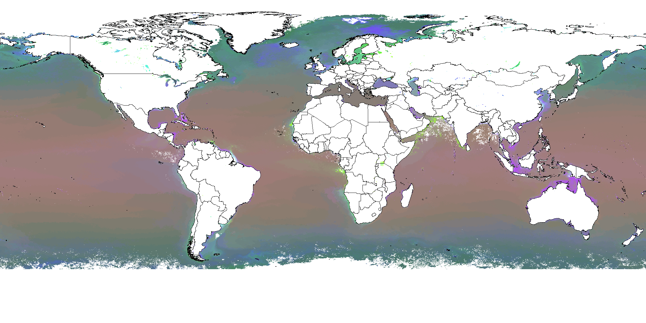When using Similarity Colors, the map is nearly indistinguishable at this scale from the one based on 1000 aquatic ecoregions colored in Similarity Colors, despite the fact that the underlying polygons in the two maps are entirely different (the earlier map has 1000 categories, while this map has 3000). This convergence to a single appearance is because both sets of quantitative aquatic ecoregions, based on the same set of input variables, are explaining the same environmental gradients. Beyond a certain level of division, both maps capture those environmental gradients adequately at a particular scale. Thus, the MGC process is not sensitive to the selection of a particular level of division, and that choice is not critical to obtaining appropriate results.

If we zoom in to a finer scale, small differences between this 3000-ecoregion set and the earliar 1000-ecoregion set may become apparent. The similarity colored aquatic ecoregions from the 3000-ecoregion set found within the Great Lakes are shown below.

A zoomed map showing the aquatic ecoregions of the Ponto-Caspian seas from the 3000-ecoregion set, shown in similarity colors.

For additional information contact:

William W. Hargrove

Oak Ridge National Laboratory

Environmental Sciences Division

Building 1507, Room 211

Mail Stop 6407

Oak Ridge, TN 37831-6407

(865) 241-2748

(865) 574-4665 fax

hnw@fire.esd.ornl.gov