|
|
Click here to obtain a PostScript version of this paper.
The authors present an application of multivariate non-hierarchical statistical clustering to geographic environmental data from the 48 conterminous United States in order to produce maps of regions of ecological similarity called ecoregions. Nine input variables thought to affect the growth of vegetation are clustered at a resolution of one square kilometer. These data represent over 7.8 million map cells in a 9-dimensional data space. For the analysis, the authors built a 126-node heterogeneous cluster--aptly named the Stone SouperComputer--out of surplus PCs. The authors developed a parallel iterative statistical clustering algorithm which uses the MPI message passing routines, employs a classical master/slave single program multiple data (SPMD) organization, performs dynamic load balancing, and provides fault tolerance. In addition to being run on the Stone SouperComputer, the parallel algorithm was tested on other parallel platforms without code modification. Finally, the results of the geographic clustering are presented.
Statistical clustering is the division or classification of a number of non-identical objects into subgroups or categories based on their similarity. Hierarchical clustering provides a series of divisions, based on some measure of similarity, into all possible numbers of groups, from one single group (which contains all objects) to as many groups as there are objects, with each object being in a group by itself. Hierarchical clustering, which results in a complete similarity tree, is computationally intensive, and the assemblage to be classified must be limited to relatively few objects. Non-hierarchical clustering provides only a single, user-specified level of division into groups; however, it can be used to classify a much larger number of objects.
Multivariate geographic clustering employs non-hierarchical clustering on the individual pixels in a digital map from a Geographic Information System (GIS) for the purpose of classifying the cells into types or categories. The classification of satellite imagery into land cover or vegetation classes using spectral characteristics of each cell from multiple images taken at different wavelengths is a common example of multivariate geographic clustering. Rarely, however, is non-hierarchical clustering performed on map cell characteristics aside from spectral reflectance values.
Maps showing the suitability or characterization of regions are used for many purposes, including identifying appropriate ranges for particular plant and animal species, identifying suitable crops for an area or identifying a suitable area for a given crop, and identifying Plant Hardiness Zones for gardeners. In addition, ecologists have long used the concept of the ecoregion, an area within which there are similar ecological conditions, as a tool for understanding large geographic areas (Bailey, 1983, 1994, 1995, 1996; Omernick, 1986). Such regionalization maps, however, are usually prepared by individual experts in a rather subjective way, and are essentially objectifications of expert opinion.
Our goal was to make repeatable the process of map regionalization based not on spectral cell characteristics, but on characteristics identified as important to the growth of woody vegetation. By using non-hierarchical multivariate geographic clustering, we intended to produce several maps of ecoregions across the entire nation at a resolution of one square kilometer per cell. At this resolution, the 48 conterminous United States contains over 7.8 million map cells. Nine characteristics from three categories--elevation, edaphic (or soil) factors, and climatic factors--were identified as important. The edaphic factors are 1) plant-available water capacity, 2) soil organic matter, 3) total Kjeldahl soil nitrogen, and 4) depth to seasonally-high water table. The climatic factors are 1) mean precipitation during the growing season, 2) mean solar insolation during the growing season, 3) degree-day heat sum during the growing season, and 4) degree-day cold sum during the non-growing season. The growing season is defined by the frost-free period between mean day of first and last frost each year. A map for each of these characteristics was generated from best-available data at a 1 sq km resolution for input into the clustering process (Hargrove and Luxmoore, 1998). Given the size of these input data and the significant amount of computer time typically required to perform statistical clustering, we decided a parallel computer was needed for this task.
Because of the geographic clustering application and other computational research opportunities, a proposal was developed which would support the construction of a Beowulf-style cluster of new PCs (Becker, et. al., 1995). With the proposal rejected and significant effort already expended, we chose to build a cluster anyway using the resources that were readily available: surplus Intel 486 and Pentium PCs destined for salvage.
|
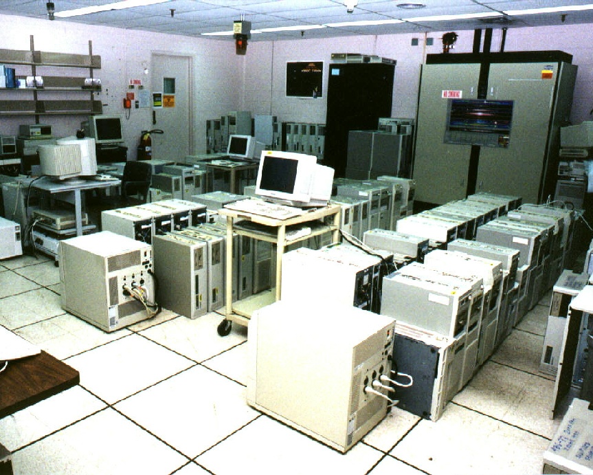
| Figure 1: The Stone SouperComputer at Oak Ridge National Laboratory. |
Commandeering a nearly-abandoned computer room and scavenging as many surplus machines as possible--from Oak Ridge National Laboratory, the Y-12 production plant, and the former K-25 site (all federal facilities in Oak Ridge)--we setup a "chop shop" to process machines and proceeded to construct a very low cost parallel computer system. Aptly named the Stone SouperComputer, after the age-old children's fable entitled Stone Soup (Brown, 1987), the heterogeneous cluster grew slowly to 126 nodes as PCs became available and were either cannabilized or fashioned into acceptable nodes. The nodes contain a host of different motherboards, processors (of varying speed and design), controllers, and disk drives. Each has 32 MB of memory, at least 400 MB of disk space (for booting and local file access), and is connected to a private 10 Mb/s Ethernet network for inter-cluster communications. In addition, one of the nodes is also connected to the external network for logins and file transfers. The system runs RedHat Linux, the GNU compilers, and the PVM and MPI message passing libraries for parallel software development (Hoffman and Hargrove, 1999; Hoffman, et. al.).
The parallel cluster, which is used for parallel program development and running models, is constantly changing. As new versions of Microsoft Windows are released, better hardware becomes available for assimilation into the cluster since users must upgrade their desktop PCs. Staying just behind the curve means the Stone SouperComputer will have a free supply of upgrades indefinitely.
The Stone SouperComputer has proven to be an excellent platform for developing parallel models which will port directly to other systems and for solving problems like non-hierarchical multivariate geographic clustering.
In our implementation of non-hierarchical clustering, the characteristic values of the 9 input variables are used as coordinates to locate each of the 7.8 million map cells in a 9-dimensional environmental data space. The map cells can be thought of as galaxies of "unit-mass stars" fixed within this 9-dimensional volume. The density of "unit-mass stars" varies throughout the data space. "Stars" which are close to each other in data space have similar values of the nine input variables, and might, as a result, be included in the same map ecoregion or "galaxy." The clustering task is to determine, in an iterative fashion, which "stars" belong together in a "galaxy." The number of clusters, or "galaxies," is specified by the user. The coordinates of a series of "galaxy" centroids, or its "centers of gravity," are calculated after each iteration, allowing the "centers of gravity" to "walk" to the most densely populated parts of the data space.
 |
| Figure 2: Clusters (or galaxies) in a 3-dimensional data space. Although the actual clusters are all roughly the same diameter, in this visualization sphere color and size are indicative of the number of map cells in each cluster (or the total mass of each galaxy if each map cell is represented by a unit-mass star). |
The non-hierarchical algorithm, which is nearly perfectly parallelizable, consists of two parts: initial centroid determination, called seed finding, and iterative clustering until convergence is reached. The algorithm begins with a series of "seed" centroid locations in data space--one for each cluster desired by the user. In the iterative part of the algorithm, each map cell is assigned to the cluster whose centroid is closest, by simple Euclidean distance, to the cell. After all map cells are assigned to a centroid, new centroid positions are calculated for each cluster using the mean values for each coordinate of all map cells in that cluster. The iterative classification procedure is repeated, each time using newly recalculated mean centroids, until the number of map cells which change cluster assignments within a single iteration is smaller than a convergence threshold. Once the threshold is met, the final cluster assignments are saved.
Seed centroid locations are ordinarily established using a set of rules which sequentially examines the map cells and attempts to preserve a subset of them which are as widely-separated in data space as possible. This inherently serial process is difficult to parallelize; if the data set is divided equally among N nodes, and each node finds the best seeds among its portion of the cells, and then a single node finds the "best-of-the-best," this set of seeds may not be as widely dispersed as a single serially-obtained seed set. On the other hand, the serial seed-finding process is quite slow on a single node, while the iterations are relatively fast in parallel. It is foolish, in terms of the time to final solution, to spend excessive serial time polishing high-quality initial seeds, since the centroids can "walk" relatively quickly to their ultimate locations in parallel. Thus, we opted to implement this "best-of-the-best" parallel seed finding algorithm. It has proven to produce reasonably good seeds very quickly.
The iterative portion of the algorithm is implemented in parallel using the MPI message passing routines--specifically, MPICH from Argonne National Laboratory (Gropp and Lusk, 1996; Gropp, et. al., 1996)--by dividing the total number of map cells into parcels or aliquots, such that the number of aliquots is larger than the number of nodes. We employ a classical master/slave relationship among nodes and perform dynamic load balancing because of the heterogeneous nature of the Stone SouperComputer on which the algorithm is run. This dynamic load balancing is achieved by having a single master node act as a "card dealer" by first distributing the centroid coordinates, and then distributing an aliquot of map cells to all nodes (Hargrove and Hoffman, 1999). Each slave node assigns each of its map cells to a particular centroid, then reports the results back to the master. If there are additional aliquots of map cells to be processed, the master will send a new aliquot to this slave node for assignment. In this way, faster and less-busy nodes are effectively utilized to perform the majority of the processing. If the load on the nodes changes during a run, the distribution of the work load will automatically be shifted away from busy or slow nodes onto idle or fast nodes. At the end of each iteration, the master node computes the new mean centroid positions from all assignments, and distributes the new centroid locations to all nodes, along with the first new aliquot of map cells. Because all nodes must be coordinated and in-step at the beginning of each new iteration, the algorithm is inherently self-synchronizing.
If the number of aliquots is too low (i.e., the aliquot size is too large), the majority of nodes may have to wait for the slowest minority of nodes to complete the assignment of a single aliquot. On the other hand, it may be advantageous to exclude particularly slow nodes so that the number of aliquots, and therefore the amount of inter-node communication, is also reduced, often resulting in shorter run times. Few aliquots work best for a parallel machine with few and/or homogeneous nodes or very slow inter-node communication, while more aliquots result in better performance on machines with many heterogeneous nodes and fast communication. Number of aliquots is a manually tunable parameter, which makes the code portable to various architectures, and can be optimized by monitoring the waiting time of the master node in this algorithm.
In order to provide some fault-tolerance, the master node saves centroid coordinates to disk at the end of each iteration. If one or more nodes fails or the algorithm crashes for some reason, the program can simply be restarted using the last-saved centroid coordinates as initial seeds, and processing will resume in the iteration in which the failure occurred.
In an effort to gauge the efficiency and scalability of the parallel clustering algorithm, a five-iteration test version of the code was developed and run, using a representative dataset of about 900,000 map cells, on a number of different architectures with two different aliquot sizes. The tests were performed on the Stone SouperComputer, an Intel Paragon XPS5, a cluster of Sun Microsystems Ultra 2 workstations, and a Silicon Graphics Inc. (SGI) Origin 2000. The test was performed using 8, 16, 32, and 64 processors where available. Tables 1 and 2 show total run times for each of these systems.
| Number of Processors |
SGI Origin 2000 |
Sun Ultra 2 Cluster |
Paragon XPS5 |
Stone SouperComputer |
|---|---|---|---|---|
| 8 | 4m 51.3s | 10m 18.4s | 1h 05m 31.3s | 30m 12.3s |
| 16 | 2m 35.1s | ------ | 17m 56.5s | 17m 05.2s |
| 32 | 1m 54.8s | ------ | 11m 33.3s | 12m 49.4s |
| 64 | ------ | ------ | 10m 15.1s | 10m 31.5s |
| Number of Processors |
SGI Origin 2000 |
Sun Ultra 2 Cluster |
Paragon XPS5 |
Stone SouperComputer |
|---|---|---|---|---|
| 8 | 5m 04.2s | 10m 32.7s | 39m 45.5s | 30m 20.1s |
| 16 | 2m 41.6s | ------ | 21m 15.6s | 16m 56.3s |
| 32 | 1m 59.0s | ------ | 10m 48.3s | 12m 52.6s |
| 64 | ------ | ------ | 6m 56.1s | 10m 34.2s |
Figure 3 shows the performance results for these machines when
naliquot=1280, i.e., 1280 is the number of aliquots or
groups into which the input data were split prior to assignment to
individual nodes. The number of iterations, that is five, was divided
by the total run time as a measure of performance and is shown on the
y-axis. Figure 4 shows similar results for
naliquot=128.
 |
Figure 3: System performance for five
iterations of the clustering algorithm for a number of parallel systems
using 8, 16, 32, 64 processors (where available) for
naliquot=1280. |
 |
Figure 4: System performance for five
iterations of the clustering algorithm for a number of parallel systems
using 8, 16, 32, 64 processors (where available) for
naliquot=128. |
For this application, the SGI significantly outperformed all the
other machines on both tests. While this tightly-coupled shared memory
environment offers excellent performance, it is an expsensive system to
purchase and maintain. Further, the largest available SGI had only 32
processors so it was not possible to obtain a result for 64
processors. Likewise, the available Sun Ultra 2 cluster was limited to
8 nodes. The 8 Sun workstations outperformed the Stone SouperComputer
and the Paragon; however, the Paragon beat the 8 Suns when using 64
processors and the Stone SouperComputer came close when using 64
processors. The Stone SouperComputer offers performance similar to the
Paragon, beating it when only 8 or 16 nodes are used. The Stone
SouperComputer beats the Paragon for small numbers of processors
because we always sort the machinefile list of nodes by
speed from fastest to slowest whenever running on the Stone
SouperComputer. The decrease in the positive slope of the performance
curve in the Stone SouperComputer is also attributable to this
fact.
With the exception of the Paragon, all machines exhibited better
performance for naliquot=1280. This implies that the
problem is not I/O bound even for 1280 aliquots.
The clustering algorithm was used to generate maps with 1000, 2000, and 3000 ecoregions. These maps appear to capture the ecological relationships among the nine input variables. This multivariate geographic clustering can be used as a way to spatially extend the results of ecological simulation models by reducing the number of runs needed to obtain output over large areas. Simulation models can be run on each relatively homogeneous cluster rather than on each individual cell. Then clustered map can be populated with the simulated results cluster by cluster, like a paint-by-number picture. This cluster fill-in simulation technique has been used by the Integrated Modeling Project to assess the health and productivity of southeastern forests.
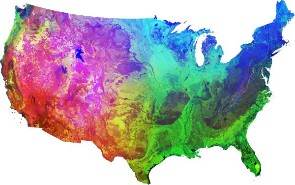 |
| Figure 5: National map clustered on elevation, edaphic, and climate variables into 3000 ecoregions using similarity colors. |
Constructing a Beowulf-style cluster from surplus equipment has proved to be well worth the effort. Unlike expensive commercial parallel systems, this kind of low-cost parallel environment can be dedicated to specific applications. We have used it to develop and run the clustering algorithm and are making it available to others who are developing and running parallel scientific models. In addition, small universities and colleges have contacted us and expressed interest in building clusters from existing machines. It is clear such "throw-away" equipment represents a hidden resource in many schools and businesses. This resource can be used thanks to the grass root efforts behind Linux, the Free Software Foundation, and academia. This kind of Beowulf-style cluster is the ultimate price/performance winner. Finally, we have demonstrated that, while special considerations, like dynamic load balancing and fault tolerance must be made for algorithms running on relatively-large heterogeneous systems, they are not difficult to implement, and result in enhanced performance on many different architectures.
mpich, a Portable Implementation of MPI."
ANL-96/6. Mathematics and Computer Science Division, Argonne
National Laboratory.
| "The submitted manuscript has been authored by a contractor of the U.S. Government under contract No. DE-AC05-96OR22464. Accordingly, the U.S. Government retains a nonexclusive, royalty-free license to publish or reproduce the published form of this contribution, or allow others to do so, for U.S. Government purposes." |